10. Jupyter and Excel
In this lecture we will talk abot:
- the relationship between Jupyter and Microsoft Excel;
- loading tables from Excel files; and
- writing tables to Excel files.
10.1. Why Jupyter, and why Excel
Microsoft Excel is the most popular spreadsheet program in the world. It owes its popularity to the fact that the table you are working on is right there in front of you, you can see it, you can click on a cell and enter a value or a formula. It is a typical representative of the What You See Is What You Get philosophy. So, why did we decide to focus this course on Jupyter?
Price. Microsoft Excel is a commercial product -- it costs money. In contrast to that Python, all of its accompanying libraries and Jupyter as the interactive environment are free of charge.
Clearly visible procedures. Data processing in Microsoft Excell consists of entering formulas into cells. If you are working with a table with intricate relationships between cells expressed by many complicated formulas spread out over the entire worksheet, it soon becomes almost impossible to track the flow of information and, more importantly, to understand, debug and improve the process. On the other hand, if the processing is expressed in terms of a programming language (such as Python), we do lose the What You See Is What You Get approach of Excel but gain much more in readability of the code. A clear procedure located in one place (a Jupyter cell or a Python file) and coded in a simple and expressive programming language can easily be checkt for errors, upgraded and shared.
Flexibility. Microsoft Excel is convenient for processing tables that are relatively small so that they can easily fit onto a few computer screens. Once you find yourself in the position where you have to process huge tables with thousands of rows and columns the advantages of scripting languages become obvious. Moreover, each Python distribution comes with a large entourage of libraries where most of the standard data processing algorithms have already been implemented.
Using clearly visible procedures that are not mingling with the data to be analyzed is the most efficient way to process data. This is the corner-stone of any approach to modern data processing.
10.2. Loading tables from local Excel files
Each Excel document consists of several worksheets. Each worksheet is a table which can be accessed through its name:
Because Microsoft Excel is the most popular spreadsheet program in the world the pandas library has a way to load a worksheet of an Excel document into a DataFrame. If an Excel document consists of several worksheets, we have to load it as several DataFrames -- one DataFrame per worksheet.
For example, the file data/Additives.xlsx has a single worksheet "E-numbers" which we load into a DataFrame straightforwardly:
import pandas as pd
additives = pd.read_excel("data/Additives.xlsx", sheet_name="E-numbers")
This file contains some basic information about additives, which are substances used in food industry to preserve food or enhance its color and taste. Let us peek at the table:
additives.head(15)
The cells that were empty in the Excel table get a special NaN value, which stands for "not a number". Since in our case these cells represent comments, we wish the empty cells to remain empty. So, we shall reload the table, but this time instruct the system not to complain about empty cells:
additives = pd.read_excel("data/Additives.xlsx", sheet_name="E-numbers", na_filter=False)
additives.head(15)
The option na_filter=False instructs the read_excel function to "switch off artificial intelligence" and leave empty cells empty. Let us make a frequency analysis based on the harmfulness of additives.
additives["Status"].value_counts()
Let us now filter the table to single out additives that may cause cancer:
additives[additives.Comment == "may cause cancer"]
Finally, let us list the additives that are marked as DANGEROUS or may cause cancer. To do so we have to combine two filtering criteria:
Comment == "may cause cancer" or Status == "DANGEROUS" (or both)
When we have to combine two criteria so that a row is included in the filtered table if at least one of the criteria is satisfied, we use the | connector:
additives[(additives.Comment == "may cause cancer") | (additives.Status == "DANGEROUS")]
10.3. Writing tables to Excel files
Any table can be written into an Excel file just like we used to write them into CSV files. The only difference is that instead ot the to_csv funcion we invoke the to_excel function. For example, let us create a table containing the list of additives that are labelled by dangerous or may cause cancer:
bad_additives = additives[(additives.Comment == "may cause cancer") | (additives.Status == "DANGEROUS")]
and let us write the table into an Excel file:
bad_additives.to_excel("data/BadAdditives.xlsx")
Let's take a look at the Excel file we've just created:
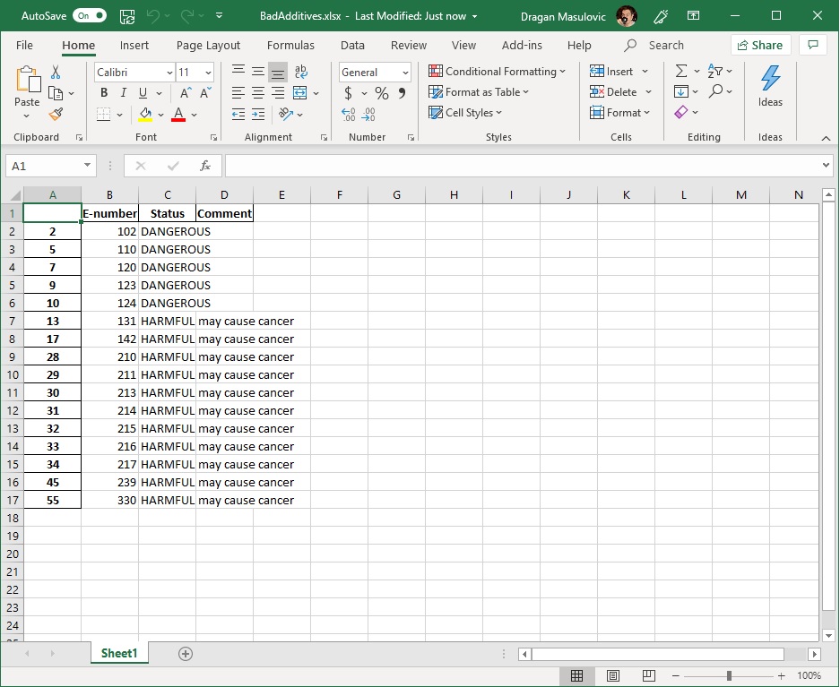
We see that the system has also written the index column of the table, which in this case is just a list of meaningless integers. To get rid of it, we'll write the table again, but this time using the option index=False:
bad_additives.to_excel("data/BadAdditives.xlsx", index=False)
The new file looks like this:
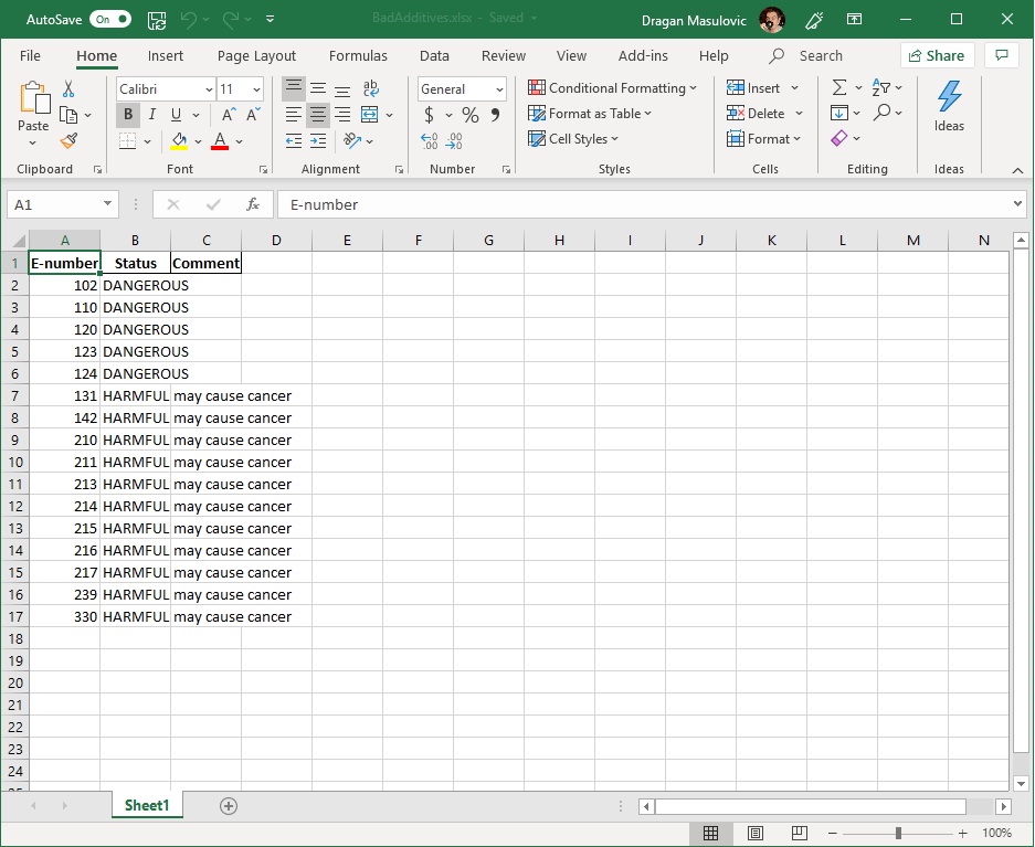
That's exactly what we wanted.
10.4. Exercises
Exercise 1. The file data/CS201.xlsx has an overview of marks of a group of students in Computer Science 201. The
data is real, so the table is anonymized.
(a) Load this table into a DataFrame and take a look at the first few rows to understand the structure of the table ("Hnn" stands for "homework nn", "Cn" stands for "colloquim n", "WE" stands for "written part of the exam" and "OE" stands for "oral oart of the exam").
(b) Index the table by "StudentID".
(c) Compute the average mark on each of the colloquia (columns "C1", "C2" and "C3").
(d) Add a new column "Avg" and for each student compute the average mark and write it into the corresponding cell.
(e) Add a new column "FinalGrade" and for each student compute the final grade based on the average mark using the following function:
def final_grade(avg):
    if avg >= 4.50:
        return 5
    elif avg >= 3.50:
        return 4
    elif avg >= 2.50:
        return 3
    elif avg >= 1.50:
        return 2
    else:
        return 1
(f) Write the new table into the Excel file data/CS201-FinalGrades.xlsx
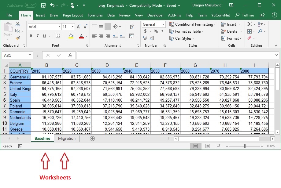
Exercise 2. Eurostat is an official European agency in charge of the statistical analyses of various data relevant to the development of the European Union. All the data Eurostat collects is publicly available at the following link: https://ec.europa.eu/eurostat/data/database
The file data/EUProjPop.xlsx contains the projection of the population of each of the EU countries 2080. The table has two worksheets: Baseline containing the projected population of the EU countries, and Migration containing the projected population of the EU countries in case of an increased migration.
(a) Load these two worksheets into to DataFrames (Baseline and Migration) and display a few rows of each table to understand the structure of the tables.
(b) Add a new row "EU" to each of the tables and compute the projected population of the entire union for each year.
(c) Add a new row to the Migration table and compute the projected migration for each of the years (subtract the row EU in the Baseline table from the row EU in the Migration table).
(d) Visualize the projected migration by a line chart.
(e) Add a new row "EU-UK" to the Baseline table and compute the projected population of EU without the UK.
(f) Write the two DataFrames to data/EU-UK.xlsx and data/EU-Migration.xlsx
Exercise 3. The file data/Cricket.xlsx contains the data about the best cricket players in the history of cricket.
(a) Load this table into a DataFrame and index it by the column "Player".
(b) Add new column "YP" (Years Played) to the table and compute the number of years of active playing for each player (subtract the column "From" from the column "To").
(c) Add new column "ARY" (Average Runs per Year) to the table and for each player compute the average number of runs per year (ARY = Runs / YP).
(d) Sort the table by "ARY" in the descending oreder and display the first 25 rows of the table. In what century were most of the top 25 players playing actively? What do you thik why?
